AOVs in RenderMan
Here, I will attempt to explain the concept of Arbritary Output variables as well as how to output these secondary images using RenderMan as well as RenderMan within Houdini.
Arbritary Output Variables are essentially extra data that can be queried from the renderer and is most often returned in image format. These images are output from secondary display channels. Note that the primary display channel returns RGBA information. The Secondary Display channel can be used to output images containing explicitly S & T co-ordinate data, Normal information, Z-depth, Point information and so on. It is highly possible that some studios output over 100 AOVs for fine artistic control in the compositing stages. I will go through a few very important ones here.
Extracting Secondary Channels
Option "searchpath" "shader" "@:../shaders"
Option "searchpath" "texture" "../textures"
Option "searchpath" "archive" "../archives:Cutter_Help/templates/Rib:custom_templates/Rib"
DisplayChannel "normal N"
Every new channel must be first declared in the rib header. It can then be rendered out to a secondary channel or to file.
Display "untitled" "it" "rgba"
Display "+/home/jburne22/Desktop/SFDM-STU-HOME/vsfx419/tiffs/untitled.t.0001.tif" "tiff" "N"
The "+" tells RenderMan that this image should be rendered through a secondary display channel. In the above case, I am going to render the AOV out to file. The file path is specified, as well as the "display driver", in this case, a .TIFF file. Then the variable "N". Global variable N tells the renderer that you are asking for surface normals.
Similarly, other AOVs may be output through secondary channels:
DisplayChannel "point P"
DisplayChannel "float s"
DisplayChannel "float t"
or when outputting images, quantization can be enabled to ensure images display on legacy devices. Quantization is an image processing technique that converts the highly detailed floating point image data format preferred by the renderer to a lower quality file format. (Color data is then stored as integer values)
DisplayChannel "t" "int[4] quantize" [0 255 0 255]Custom AOVs
The usefulness of AOVs is most emphasised with the ability to export powerful custom AOVs using shaders. Here is an example of how Depth was exported using a shader:
surface { zdepth = depth(P); /*float zdepth = depth(P);* << do not declare a variable like this. It is only local, /* STEP 1 - set the apparent surface opacity */ /* STEP 2 - calculate the apparent surface color */ |
Here, the value of the depth(P) function is stored in a variable called zdepth. The value of "P" is measured by calculating the distance from the camera (z axis) to the each shaded point on the primitive.In my shader above, I went through the extra step of adding the result of zdepth to my "surfcolor", which eventually lets zdepth be the apparent color of my surface. One can se the result of that on my LOD Displace page. A barebones zdepth shader may look like this:
surface zdepth = 1 - depth(P); |
The result of this shader may be exported through a secondary display channel. First the Display channel is declared in the rib header:
DisplayChannel "float zdepth"
Then initialize the secondary channel:
Display "+/[file path]/untitled.zdepth.0001.tif" "it" "zdepth"
Specialized Custom AOVs
In this example, a shader is used to query the light for information. That information is then stored in an AOV. This example illustrates how very specific AOVs may be exported for unique situations.
surface
diffuse_test(float Kd = 1;
output varying float __shadow = 0;
output varying float __inshadow = 0;
output varying color __no_shadow_ci)
{
color surfcolor = 1;
Here, all the variables are declared. The values stored in these varying floats will be used later to generate specific AOVs.
normal n = normalize(N);
vector nf = faceforward(n, I);
Oi = Os;
float shad = 0;
color totalLightColor = 0;
The normal of each point is "normalzied", or explicitly set to 1 from whatever value it was before. It is a good habit to initalize normals to 1, since many mathematical operations depend on this value for accuracy.
Variable vector nf is not used in this shader, but here in this example, it stores the value of the faceforward() function. According to the pixar documentation, this function flips the normal, so that it points opposite to the direction of the incident ray (I).This is important since the color contribution from a single light is directly proportional to Ln.Nf (the dot product between the normalized Light direction and the surface normal)
illuminance(P, n, PI) { .... arguments ... }Illuminance() is an interesting function that dictates how much a light gets to contribute to shading a surface, if it gets to contribute at all.It is best illustrated using a diagram.
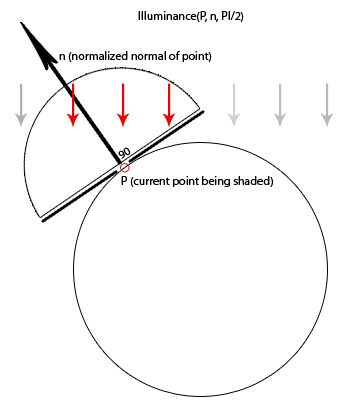 |
Here, I illustrate the operations of Illuminace(P,n,PI/2). Given all the lights in a scene, the statements in the body of an illuminance() block are executed just for those lights that meet the criteria specified within the parentheses.First, the function asks for P, the location of the current point being shaded.It uses P as the center of a sphere with respect to which lights are to be used.The next is the Normal, which will be used as an axis and PI/2, which is an angle measured in radians. PI/2 is 90 degrees. This leads to a hemisphere centered at P (current point being shaded). Only the lights that fall within this "illuminance cone" will be considered for the calculations inside the illuminance block.I illustrate this with arrows representing different lights. One can clearly see the grey rays fall out of the illuminance cone, hence they will not contribute to the light calculations. Only the red rays will contribute to the shading of point P. |
In the case of our shader, here is the information that we put inside the illuminance loop:
//Query the current light for the value//of it's output parameter
if(lightsource("__inshadow",shad) == 1)
__shadow += shad;
// Same again for the light color that was
//not darkened by a shadow
color cl = 0;
if(lightsource("__cl_noshadow", cl) == 1)
totalLightColor += cl * normalize(L).n;
//Are we in the "self shadowing" part
//of the surface??
float dot = n.normalize(-L);
if(dot >= 0)
__shadow = 1;
diffusecolor += Cl * normalize(L).n;
}
Here, a function called lightsource() is used to query the output of a light. In the case of:
if(lightsource("__inshadow",shad) == 1)
__shadow += shad;
The value of "__inshadow" is stored in the variable "shad". If that value equals to 1, then "__shadow" variable, previously set to 0, will now equal to 0 + "shad" (0 + 1). So this __shadow variable used as an AOV will now only output what is in shadow. We can constantly query what is in shadow and what is not by using this lightsource() function and output the results to AOVs.
For the other part of the shader, we query the part of the sphere not receiving light. Generally, to calculate which point is currently in shadow would be to get the cosine of the angle between Ln (light ray direction) and Nn (normal). The dot product is always equivalent to the cosine of two normalized angles. One also sees from the Illuminance illustration that when using PI/2, any angle that goes between 0 to 90 degrees will mean head-on to sideways illumination. Cos(0 degrees) = 1 and Cos(90 degrees) = 0. The "if" statement says "if (dot >= 0) then __shadow = 1". The only way the dot product could go into a negative is if the Ln.Nn angle is greater than 90 degrees, which subsequently means that according to the Illuminance (PI/2) function, that point will not get shaded. It is also interesting to note that cos(180 degrees) is equal to -1. So we can use that last "if" statement to get the result of shadowed areas.
See complete SL code here.
Next, you would have to construct a light shader that this surface shader queries for some values.
See the complete SL code for the light shader here.
Interesting points to note about the light shader:
solar(direction, 0.0)Quite different from the Illuminance function, in the sense that the solar() function is used to specify distant light sources either along a given direction or along all directions. Light rays shot from the illuminate cone (also a 3-dimensional cone) of the light source shader are parallel and shines from infinity, which is why a point position is not needed in this function.
if(shadowname != "") {
__inshadow = shadow(shadowname, Ps,
"samples", Shading_samples,
"width", Sample_width);
Cl = mix(lightcolor, shadowcolor, __inshadow) ;
}
This statement states that if the user specified a shadow map, pass that shadow map to the shadow() function to initialize the shadow. The shadow function also allows the user to specify shading samples to fine tune the look. Overall shadow color is mix of the lightcolor, shadowcolor and shadow map.
//if(gel != "")// Cl = Cl * texture(gel);
}
Declaring and outputting these secondary channels in RIB are as follows.
In the RIB header specify:
DisplayChannel "float __shadow" "quantize" [0 65535 0 65535]DisplayChannel "float __inshadow" "quantize" [0 65535 0 65535]
DisplayChannel "color __no_shadow_ci" "quantize" [0 65535 0 65535]
Then output the information to secondary channels:
Display "simple_distant" "it" "rgba"Display "+simple_distant.__shadow" "it" "__shadow"
Display "+simple_distant.__selfshadow" "it" "__inshadow"
Display "+simple_distant.__no_shadow_ci" "it" "__no_shadow_ci"
Declare the custom light source:
LightSource "simple_distant_lightLookup" 2 "intensity" 1"shadowname" ["distant_map.tex"]
# "gel" ["swazi.tex"]
Apply the custom shader to a simple primitive:
Surface "diffuse_test"TransformBegin
Translate 0 0.35 0
Scale 0.15 0.15 0.15
ReadArchive "nSphere.rib"
TransformEnd
See the complete RIB here.
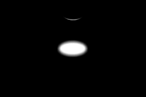
 Object with Shadows |
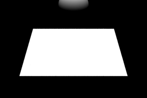 AOV Excluding Shadow |
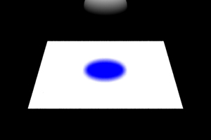
 AOV showing Self Shadow Pass |
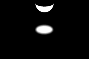 AOV showing Full Shadowed Area |